

Database system
导航
- 导航
- introduction
- chapter2-Relational Model
- chapter3-introduction to SQL
- chapter4-intermediate SQL
- chapter5-advanced SQL
- chapter6-E-R Model
- chapter7-Relational Database Design
- chapter13-Data storage structures
- chapter14-Indexing
- chapter15-Query Processing
- chapter16-Query Optimization
- Chapter 17-Transactions
- Chapter 18-Concurrency Control
introduction
purpose of database system
- 早期database application建立在file systems上有data redundancy,data isolation,difficulty in accessing data等问题。
- integrity problems(完整性问题)
在数据库中integrity constraints can be stated explicitly. - Atomicity problems(原子性问题)
在数据库中主要通过恢复功能来解决原子性问题。 - concurrent access anomalies(并发访问异常)
对于并发操作若不采取任何限制,可能会导致数据混乱。 - Security problems
数据库系统提供以上问题的解决措施。
Characteristics of Databases
- data persistence
- convenience in accessing data
- data integrity
- data security
- concurrency control for multiple users
- failure recovery
view of data
- 三级抽象databases(Hide the complexities,enhance the adaptation to changes)
- 主要通过两层map来体现数据库的物理数据独立性和逻辑数据独立性。
- view level
- logical level
- physical level
data Models
most important:Relational Model
Database languages
Data Definition Langauge(数据定义语言)
- DDL compiler generates a set of table templates stored in a data dictionary
- Data dictionary contains metadata
Data Manipulation Language(数据操作语言)
SQL:widely used non-procedural language(陈述式语言)
1
2
3
select name
from instructor
where instructor.ID = '12345'
Database Design
- Entity Relationship Model(实体-联系模型)
- Normalization Theory
Database Engine
Storage manager
chapter2-Relational Model
Basic Structure
- 定义:Formally, given sets D1, D2, …. Dn a relation r is a subset of D1 x D2 x … x Dn.Thus, a relation is a set of n-tuples (a1, a2, …, an) where each ai $\in$ Di。也就是说虽然我们可视化展示的是一个列表,但是本质是没有顺序的,因为是一个集合。
- A1,A2….An are attributes
- R=(A1,A2,..,An) is a relation schema
- Database shcema – is the logic structure of the database.
Attributes
- The set of allowed values for each attribute is called the domain(域) of the attribute.
- 通常值是原子的.
- 在数据库中为每一个域都规定了相同的空值.
keys
- 定义:K$\in$R.K is a superkey(超健) of R if values for K are sufficient to identify a unique tuple of each possible relation r(R).
- Example: {ID} and {ID,name} are both superkeys of instructor.(但是名字不是,因为存在重名的情况)
- Superkey K is a candidate key(候选健) if K is minimal.
- Example: {ID} is a candidate key of instructor.
- One of the candidate keys is selected to be the primary key(主键).
- Foreign key(外键) constraint from attribute(s) A of relation r1 to the primary key B of relation r2 states that on any database instance, the value of A for each tuple in r1 must also be the value of B for some tuple in r2. (参照完整性,类似于外键限制,但是并不一定局限于主键)

解释:由上面的例子,第三排的course中的dept_name就是外键,因为course中的dept_name和department中的dept_name(是主键)是同一个值,所以course中的dept_name就是外键。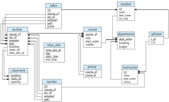
解释:红色箭头表示参照完整性,黑键则表示外键。
Relational Algebra
- 输入几个关系,通过某个操作得到一个新的关系。
- Six basic operations:
- select(横向选择)$\theta$
- project(投影某几列,并且结果会去重)$\pi$
- union(对两个关系并起来)
- 两个关系必须有相同的元数(same number of attributes)
- attributes的域需要相容
- set difference -
- 笛卡尔积(表的乘积) x
- rename $\rho$ (当对一个关系想做笛卡尔积的时候,可以对其改名再执行笛卡尔积)
Additional Operations
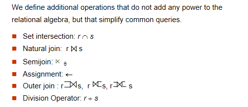
- 自然联结的例子
- 除法操作
- 结果里面的元组与除数元组连接一定在被除的关系中
Extended Relational-Algebra-Operations
Generalized Projection
Aggregate Functions
chapter3-introduction to SQL
Data Definition Langauge
Domain Types in SQL
- char(n). Fixed length character string, with user-specified length n.(与C语言有差异,因为C语言的字符串的结尾一定为\0,它以字符数组的形式存储,而数据库作为字典直接可以从存储中截取对应长度,不需要额外的标识符)
- varchar(n). Variable length character strings, with user-specified maximum length n.
- int. Integer (a finite subset of the integers that is machine-dependent).
- smallint. Small integer (a machine-dependent subset of the integer domain type).
- numeric(p,d). Fixed point number, with user-specified precision of p digits, with d digits to the right of decimal point.
→ number(3,1) allows 44.5 to be store exactly, but neither 444.5 or 0.32 - real, double precision. Floating point and double-precision floating point numbers, with machine-dependent precision.
- float(n). Floating point number, with user-specified precision of at least n digits.
Built-in Data Types in SQL
- date
- time
- timestamp(data plus time of day)
- interval(period of time)
Create Table Construct
1 | |
- 再研究key
- not null
- primary key(A1,…,An)
- foreign key(Am,…An) references r(对于被引用的表如果发生delete或者update,可以进行这四个操作:cascade(那个表的值怎样变,此表的值就怎么变), restrict(限制不变), set null, set default)
- 总结对比
- 操作类型 描述 示例场景
- CASCADE 被引用表数据变化时,当前表相关数据自动同步变化。 删除部门时自动删除员工记录
- RESTRICT 如果当前表有依赖数据,则拒绝被引用表的数据变化。 防止删除仍有员工的部门
- SET NULL 被引用表数据变化时,当前表相关外键字段被设置为 NULL。 删除部门时将员工的部门字段置空
- SET DEFAULT 被引用表数据变化时,当前表相关外键字段被设置为默认值。 删除部门时将员工的部门字段设为默认
1 | |
Basic Query Structure
The select clause
- SQL 大小写不分的
- find the names of all instructors
- select name
- from instructor
The from clause
- The from clause lists the relations involved in the query
- Corresponds to the Cartesian product operation of the relational algebra
Natural join example
1 | |
string operations
Ordering the display of tuples
1 | |
Aggregate Functions
- 聚合函数的使用
- 直接使用聚合函数:适用于对整个表或满足某些条件的数据进行聚合操作。
- 结合 GROUP BY 使用聚合函数:适用于按某个字段分组后对每组分别进行聚合操作。
- 因此,是否需要 GROUP BY 取决于具体的业务需求。如果只是对整体数据进行统计,无需分组;如果需要按某些字段分组统计,则必须使用 GROUP BY。
1 | |
group by clause
- 当我们使用group by的时候是一个聚合操作,所以最终的的select的结果也是以组的形式存在
- ex
![group]()

having clause
1 | |
Nested Subqueries
Set membership
- 通过in和not in来实现嵌套操作
1 | |
set comparison
- 利用some和all与给定集合进行比较
1 | |
test for empty relations
- 利用exists和not exists
1 | |
Test for
Modification of the Database
chapter4-intermediate SQL
joined relations
- join types
- inner join(默认的笛卡尔积均是inner join)
- left outer join(from后面的表的所有列均保留,如果没有成功连接上,则置为NULL)
- right outer join(join后面的表的所有列均保留)
- full outer join
- join conditions
- natural join(自然连接)
- on condition(条件连接)
- using(A1,…,An)(等值连接)
- example
- 统计每个老师教的课程(但是可能包含没有课程的老师)
- select id,count(course_id)
- from instructor natural left outer join teaches
- group by id;
- 统计每个老师教的课程(但是可能包含没有课程的老师)
SQL Data Types and schemas
User-defined types
- create type construct in SQL creates user-defined type
- create type Dollars as numeric(12,2) final
domains
- domain is a user-defined type that specifies a set of values and a set of constraints on the values in the set.domains相比于types,domain可以定义一些约束,比如长度,范围,正则表达式等。
- craete domain person_name char(20) not null
integrity constraints
Not NULL and Unique constraints
the check clause
views
- A view provides a mechanism to hide certain data
from the view of certain users.(虚拟的表,没有实际存在) - 好处:简化复杂性,适应能力增加,提供安全权限管理功能。
example views
- a view of instructors without their salary
- create view faculty as
select ID, name, dept_name
from instructor; - 当我们创建好这个view以后,我们可以把这个view当作实体的表进行表的各种操作
- create view faculty as
views defined using other views
- 在定义view的基础上,可以再定义一个view
- create view physics_fall_2009 as
select course.course_id, sec_id, building, room_number
from course, section
where course.course_id = section.course_id
and course.dept_name = ’Physics’
and section.semester = ’Fall’
and section.year = ’2009’; - create view physics_fall_2009_watson as
select course_id, room_number
from physics_fall_2009
where building= ’Watson’; - 这样的操作其实我们可以在一个语句中实现
select course_id, room_number
from physics_fall_2009(已经创建的view)
where building= ’Watson’;
→
select course_id, room_number
from (select course.course_id, building, room_number
from course, section
where course.course_id = section.course_id
and course.dept_name = ’Physics’
and section.semester = ’Fall’
and section.year = ’2009’)(把view创建的语句嵌套在from中)
where building= ’Watson’;
→
select course_id, room_number
from course, section
where course.course_id = section.course_id
and course.dept_name = ’Physics’
and section.semester = ’Fall’
and section.year = ’2009’
and building= ’Watson’;(sql本质运行的一种语句)
update of a view
- view相当于只是打开一扇窗,所以对view的修改,实际上是对view的表进行修改。当然孙老师说,为了提高查询的高效性,有些时候确实会创建一个临时表(materialized view)。
- example
insert into faculty values (’30765’, ’Green’, ’Music’);
insert into instructor values (’30765’, ’Green’, ’Music’, null); - 但是有些时候view的update不能被翻译为对原始表的独立的操作,因为这个view选取的元素可能不是超键。
view and logical data dependence
- 当我们底层的物理数据发生变化,比如一个表分成了两个表,因为我们用户层面可能用到原来的表,那么我们可以利用现在的两个表生成一个代表原来表的view,对于用户层面没有任何变化,但是底层逻辑发生改变。
Indexes
transactions(事务)
- 在数据库系统中,事务是指一组操作的集合,这些操作要么全部执行成功,要么全部不执行,以确保数据的一致性和完整性。
transaction properties
- 原子性(Atomicity):事务是一个不可分割的工作单位,事务中的所有操作要么都做,要么都不做。
- 一致性(Consistency):事务必须使数据库从一个一致状态变换到另一个一致状态。如果事务执行成功,则数据库处于一致状态;如果事务执行失败,则数据库应恢复到事务开始前的状态。
- 隔离性(Isolation):多个事务并发执行时,一个事务的执行不应影响其他事务的执行结果。每个事务都应该独立运行,就好像它是唯一正在运行的事务一样。
- 持久性(Durability):一旦事务提交,它对数据库的更改应该是永久性的,即使系统发生故障。
transaction example
SET AUTOCOMMIT=0;
UPDATE account SET balance=balance -100 WHERE ano=‘1001’;
UPDATE account SET balance=balance+100 WHERE ano=‘1002’;
COMMIT;(上一条事务结束,下一个事务开始)
UPDATE account SET balance=balance -200 WHERE ano=‘1003’;
UPDATE account SET balance=balance+200 WHERE ano=‘1004’;
COMMIT;
UPDATE account SET balance=balance+balance*2.5%;
COMMIT;
transaction operation
- BEGIN TRANSACTION; 或 START TRANSACTION;:显式地开始一个新的事务。
- COMMIT;:提交当前事务,使其所有更改永久生效。
- ROLLBACK;:回滚当前事务,撤销所有未提交的更改,是数据库恢复到事务开始之前的状态。
- SAVEPOINT savepoint_name;:设置一个保存点,可以在部分回滚时使用。
- ROLLBACK TO savepoint_name;:回滚到指定的保存点,而不是整个事务。
Autorization(授权)
- the grant statement is used to confer authorization:grant (privilege list) on (relation name or view name) to (user list)
- user list:
- user-id
- public,which allows all valid the privilege granted
- a role(more on this later),作用周期是永久性的,角色也就是用户的集合,可以创建角色,然后给角色授予权限。
privileges in SQL
grant select on instructor to U1, U2, U3
grant select on department to public
grant update (budget) on department to U1,U2
grant all privileges on department to U1
- the revoke statement is used to revoke authorization:revoke (privilege list) on (relation name or view name) from (user list)
chapter5-advanced SQL
Accessing SQL from a programming language
- two approaches to access database
- API
- Embedded SQL
API
- ODBC works with C,C++,C#
- JDBC works with Java
- Open a connection
- Create a “statement” object
- Execute queries using the Statement object to send queries and fetch results
- Exception mechanism to handle errors
- Embedded SQL in C
- SQLC-embedded SQL in Java
- JPA-OR mapping of Java
JDBC
JDBC code
1 | |
Prepared Statement
- 先生成,类型未知,再利用set语句和update语句进行更新
- prepared statement也可以避免SQL注入攻击,因为我们提前进行编译,就会防止产生SQL的歧义。
1 | |
Metadata
- JDBC可以利用getMetaData()方法来获取数据库的元数据,比如列名,列类型,列数目等。
ODBC(open database connectivity)
ODBC Code
- 完全通过函数调用实现
1 | |
main body
1 | |
ODBC prepared statements
Embedded SQL
procedural constructs in SQL
SQL functions
- 定义函数后再调用
1 | |
SQL procedures
1 | |
Triggers
- A trigger is a statement that is executed automatically by the system as a side effect of a modification to the database.
- ECA rule
- Event: A modification to the database(insert,delete,update)
- Condition: A condition that must be satisfied for the trigger to execute
- Action: An action to be performed when the condition is satisfied
Trigger example
1 | |
Statement Level Triggers
chapter6-E-R Model
E-R Diagram
- section:弱实体,自己的属性不能表示唯一的实体,所以通过sec_course等relationship,则可以表示section依赖course等,就能够唯一确定section。我们也发现section的某个属性下方为虚线,它需要与它所依赖的主键组合起来成为主键。
chapter7-Relational Database Design
deposition
- 因为我们想要获得更小的表,所以要将原来的relation进行分解,但是此时分解存在两种情况:
- lossy decomposition: 丢失一些信息,分解后的表通过natural join以后不能重构得到原来的表。
- lossless decomposition:$\pi_{R_1}(r) \natural \pi_{R_2}(r) = r $
- lossless decomposition的充要条件是至少满足以下两个条件之一:R1与R2的交集为R1的超键,或者R1与R2的交集为R2的超键。
chapter13-Data storage structures
File Organization
Fixed-length records
- 所有记录的长度都相等,当发生删除时:
- move records i + 1, . . ., n to i, . . . , n – 1
- move record n to i
- do not move records, but link all free records on a free list
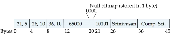
Variable-length records
- Attributes are stored in order
- Variable length attributes represented by fixed size (offset, length), with actual data stored after all fixed length attributes
- Null values represented by null-value bitmap(空位图)
![database1]()
解释:这上面是一个例子,不定长的保存在后面,定长的与(offset,length)保存在前面。在这个例子中,null bitmap表示前面四个属性都是非空的。 - 存储variable-length records采用slotted page structure,whose header contains:
- number of record entries
- end of free space in the block
- location and size of each record
- 需要注意的是:Records can be moved around within a page to keep them contiguous with no empty space between them; entry in the header must be updated.
Record pointers should not point directly to record — instead they should point to the entry for the record in header.
Organization of records in files
- heap:有空余位置就插入
- 每一个block都有一个entry,维护一个空闲块地图,记录这个块的空闲程度。
- sequential:插入元素维护一个次序
- In a multitable clustering file organization records of several different relations can be stored in the same file。
- Motivation: store related records on the same block to minimize I/O
- B+tree file organization
- Hashing
chapter14-Indexing
Basic Concepts
Ordered Indices
- Primary index:in a sequentially ordered file, the index whose search key specifies the sequential order of the file.
- Secondary index(辅助索引): an index whose search key specifies an order different from the sequential order of the file. Also called non-clustering index.
- Dense index(稠密索引) — Index record appears for every search-key value in the file.
- Sparse Index(稀疏索引): contains index records for only some search-key values.
B+-Tree Index
properties of B+-tree
- All paths from root to leaf are of the same length
- Inner node(not a root or a leaf): between [n/2] and n children.
- Leaf node: between [(n–1)/2] and n–1 values
- Special cases:
- If the root is not a leaf:
at least 2 children. - If the root is a leaf :
between 0 and (n–1)values.
- If the root is not a leaf:
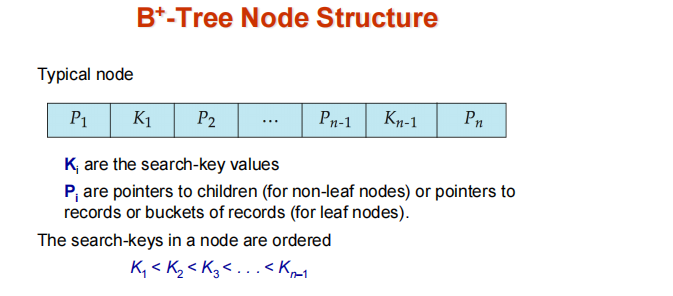
B+-Tree Node Structure
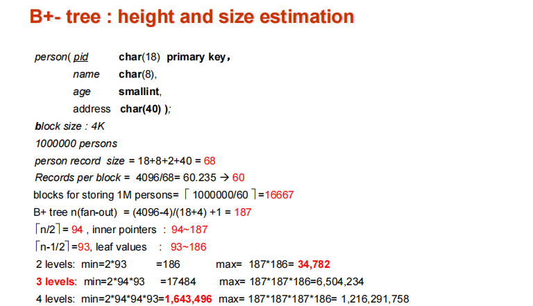
B+-tree:height and size estimation
- 最关键的是找到fan-out,因为按照我们上面提到的B+Tree Node structure,每一个fan都是由serch key和指针决定。我们的fan_out就是由search key和指针的大小以及block size决定。
Indexing strings
- 如果索引值为variable length strings,按照前面的思路我们可能得到不同的fanout。
- 解决:采用前缀压缩解决
Non-Unique Search keys
B+-File Organization
- B+-Tree File Organization:
- Leaf nodes in a B+-tree file organization store records, instead of pointers
- Helps keep data records clustered even when there are insertions/deletions/updates
- Leaf nodes are still required to be half full
- Since records are larger than pointers, the maximum number of records that can be stored in a leaf node is less than the number of pointers in a nonleaf node.
- Insertion and deletion are handled in the same way as insertion and deletion of entries in a B+-tree index.
Indices on Multiple Keys
- Composite search keys are search keys containing more than one attribute。
- 大小的比较就根据属性的次序依次比较即可
Bulk Loading and Bottom-Up Build
- 将条目逐个插入B+树中,假设叶级无法装入内存,则每次需要1 IO,对于一次加载大量条目(批量加载)来说,这可能非常低效
- 选择1:insert in sorted order
- 选择2:Bottom-up build
- 首先把所有索引排序
- 从叶子节点开始向上构造每一层
- The built B+-tree is written to disk using sequential I/O operations
- 如果要批量插入较大规模的数据,我们可以直接合并为大的b+tree,然后使用bottom-up build方法构建。(其中原来的b+tree在磁盘中是连续存放的,所以我们归并时只要seek1次,然后连续读入block进行归并。最后构建好b+tree后再seek1次,并且通过block transfers写入磁盘)
Indexing in Main Memory
- Random access in memory
- Much cheaper than on disk/flash, but still expensive compared to cache read
- Binary search for a key value within a large B+-tree node results in many cache misses
- Data structures that make best use of cache preferable – cache conscious
- 小节点的b+树适合缓存行的树比减少缓存缺失更可取
- 总结:优化磁盘访问采用大节点;优化缓存采用小节点的树,减小cache miss.
Indexing on Flash
- Random I/O cost much lower on flash
- Write-optimized tree structures (i.e., LSM-tree) have been adapted to minimize page writes for flash-optimized search trees
Write optimized indices–优化B+树
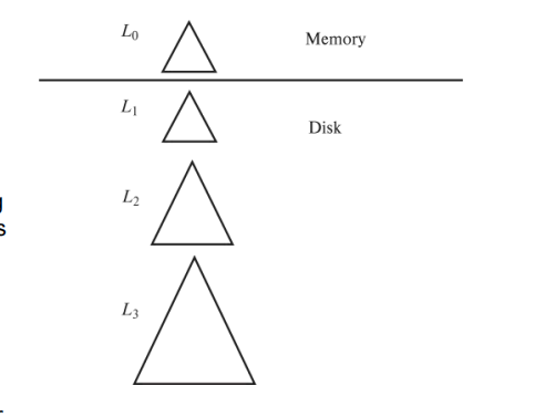
Log Structured Merge Tree
- 结构
![database143]()
- records inserted first into in-memory tree(L0 tree)
- 内存里的B+tree满了的话,就写入磁盘中。此时b+tree的构建如果使用L0和L1就可以采用自下而上的构建方式。
- 当L1超过某个阈值以后merge into L2,并且新树的阈值是原来树的阈值的倍数。
- benefits
- 减少IO次数,减少磁盘碎片化。
- 始终顺序I/O操作。因为当使用LSM Tree的时候,数据先写到内存,满了再到磁盘,磁盘分级向下,始终是一个顺序的操作。
- drawbacks
- 查询必须搜索多棵树
- 内容都要复制多次(因为merge的缘故)
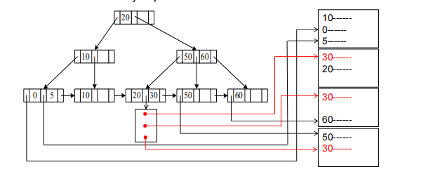
- stepped merge index
- 是传统的LSM tree的变体,每一个level在磁盘上都有k棵树。当k个索引处于同一层时,合并得到一颗层数加一的树。
- 所以我们通过延迟merge,使得写入更便宜,但是查询变得更贵了。
- 优化查询的一个方法是使用Bloom filter
- 给每棵小树都配一个 Bloom Filter。查询一个 key 时,先检查 Bloom Filter,只有 Bloom filter 返回可能存在,才真正去访问磁盘文件。如果 Bloom filter 说肯定不存在,就可以跳过这个树,省下一次磁盘 I/O。
buffer tree
- 主要思想:B+树的每个内部节点都有一个缓冲区来存储插入
- 当缓冲区满时,插入操作将移动到较低级别。使用大缓冲区时,每次都会将许多记录移动到较低级别。每条记录的I/O会相应地减少
chapter15-Query Processing
Basic steps in query processing
- by parser and translator to relational algebra expression
- amongst all equivalent evaluation plans choose the one with the lowest cost
- evaluation of the chosen plan
measures of query cost
- 为了简便计算,我们只考虑number of transfeers and the number of seeks.
- cost for b block transfers plus S seeks:$b * t_T+S * t_s$
selection operation
file scan
- 线性扫描,Scan each file block and test all records to see whether they satisfy the selection condition.
worst cost = br * tT + tS(假设连续存放,则只需要进行一次seek)br denotes number of blocks containing records from relation r - If selection is on a key attribute, can stop on finding record average cost = (br /2) tT + tS(如果数据没有连续存放则不能进行二分查找)
selection using indices
- Index scan – search algorithms that use an index
- A2 (primary B+-tree index / clustering B+-tree index, equality on key). Retrieve a single record that satisfies the corresponding equality condition. Cost = (hi + 1) * (tT + tS)
- A3 (primary B+-tree index/ clustering B+-tree index, equality on nonkey) Retrieve multiple records. Records will be on consecutive blocks. Cost = hi(tT + tS) + tS + tT* b
- A4 (secondary B+-index on nonkey, equality).
Each of n matching records may be on a different block.(指针对应的记录) n pointers may be stored in m blocks. Cost = (hi + m+ n) * (tT + tS)![database151]()
selections involving comparisons
- A5 (primary B+-index / clustering B+-index index, comparison). (Relation is sorted on A)
- For $\rho_{A \ge v}(r)$ use index to find first $tuple \ge v$ and scan relation sequentially from there. Cost is identical to the case of A3 → Cost=hi*(tT + tS) + tS + tT* b
-For $\rho_{A \le v}(r)$ just scan relation sequentially till first tuple > v; do not use index - A6 (secondary B+-tree index, comparison). $\rho_{A \ge v}(r)$ use index to find first index $entry \ge v$ and scan index sequentially from there, to find pointers to records.
- $\rho_{A \le v}(r)$ just scan leaf pages of index finding pointers to records, till first entry > v
sorting
external sort-merge(比较重要)
- Let M denote memory size (in pages).Total number of runs : [br /M].Total number of merge passes required: log M–1(br/M).Block transfers for initial run creation as well as in each pass is 2br.
- Cost of seeks: (simple version) During run generation: one seek to read each run and one seek to write each run.2[br / M].During merge passes: one seek to read each run and one seek to write each run.Total number of seeks:2 [br / M] + br (2 [logM-1(br / M)] -1)
- advanced version
- 思想:1 block per run leads to too many seeks during merge Instead use bb buffer blocks per run:read /write bb blocks at a time.
- Total number of merge passes required: log [M/bb]–1(br/M)
join operations
Nested-Loop Join
- 在这个算法的情况下,我们利用循环嵌套逐个检查每一个tuple,每个tuple和每个tuple配对检查。
- In the worst case, if there is enough memory only to hold one block of each relation, the estimated cost is nr*bs+ br block transfers, plus nr+ br seeks
(注意内存对于每个关系只能放一个block,所以每次外关系从磁盘传进内存,所以每次都要seek,总的为br seeks。而当外关系seek进来以后,每一个外关系的tuple都对应需要seek一次的内关系,然后进行block transfers) - 如果内存足够大,能够将关系全部放入内存,block transfers:br+bs block seeks:2
block nested-loop join
- 这个是循环嵌套的变体,我们首先将外关系的block与内关系的block配对,再在block内进行tuple的遍历配对。(所以算法会显示有四层循环)
- worst case:$br * bs+ br$ block transfers $ + 2*br$ seeks(和循环嵌套相比,因为我们站在block的视角,所以将nr替换为br)
- Use M-2 disk blocks as blocking unit for outer relations, where M = memory size in blocks; use remaining two blocks to buffer inner relation and output.
- Cost = [br / (M-2)] * bs + br block transfers + 2 [br / (M-2)] seeks.如果块的数量很多,那么cost=bs+br block transfers +2 seeks
indexed nested-loop join
- 如果连接是等值连接或自然连接并且内关系的连接属性上存在索引,则索引查找可以替代文件扫描可以构建索引来计算连接。对于外关系r中的每个元组$t_r$,使用索引查找满足与元组$t_r$的连接条件的s中的元组。
- Cost of the join: br(tT + tS) + nr*c(其中c是遍历索引和获取一个元组或r的所有匹配s元组的成本)
merge-join
- 只能适用于等值连接和自然连接(因为merge-join的操作核心就是基于关系之间链接的属性进行排序)
- Each block needs to be read only once. assuming all tuples for any given value of the join attributes fit in memory.Thus the cost of merge join is: br + bs block transfers +[br/ bb]+ [bs/ bb]seeks(注意bb指的是缓冲块数,通常情况为1)
- 其实从最后的cost结果我们可以反过来发现,merge-join的本质其实就是通过sorted来减少我们比较的次数,从而减少transfers的次数。
- 假如buffer memory size为M pages,最小化cost:$br+bs+[br/x_r]+[bs/x_s] (x_r+x_s=M)$ answer:$x_r=\sqrt{b_r}*M/(\sqrt{b_r}+\sqrt{b_s});x_s=\sqrt{b_s}*M/(\sqrt{b_r}+\sqrt{b_s})$
hash join
- Applicable for equi-joins and natural joins.
- 基本原理:
- 哈希连接的核心思想是使用哈希表(Hash Table)来加速连接操作,其基本步骤分为两个阶段:
- 构建阶段(Build Phase):
- 选择较小的表(称为构建表,Build Table)作为输入。
- 对连接列计算哈希值,并构建哈希表(通常存储在内存中)。
- 探测阶段(Probe Phase):
- 扫描较大的表(称为探测表,Probe Table)。
- 对探测表的连接列计算哈希值,并在哈希表中查找匹配项。
- 如果找到匹配,则输出连接结果。
- 分区哈希连接
- 分区阶段:对构建表和探测表按照哈希值进行分区,再写入磁盘
- 连接阶段:逐个加载分区到内存,进行哈希连接
- cost of hash-join
- 不需要recursive partition:$3 * (b_r+b_s)+4 * n_h$ block transfers+$2 * ([b_r/b_b]+[b_s/b_b])+2 * n_h$ seeks
- 解释:首先在分区阶段,我们从磁盘读入,分区后再写入消耗$2*(b_r/b_b+b_s/b_b)$ seeks,$2*(b_r+b_s)$ block transfers;在构建和探测阶段,逐个加载分区$b_r+b_s$ block transfers,分区占用的块数可能略多于br +bs,这是由于部分填充的块所致。访问这些部分填充的块可能会为每个关系增加最多2nh的开销,因为每个nh个分区中都可能存在一个需要写入和读回的部分填充块。
- recursive partitioning
- 如果分区数n大于内存页数M,则需要递归分区(不再使用n个分区,而是使用M-1个分区来处理s。再使用不同的哈希函数对M-1个分区进行进一步划分。同样的方式处理关系r)
- 所以我们可以得到不使用recursive时的条件:$M \ge \frac{b_s}{M}+1=n_h+1$(在这里我觉得前面的表述存在问题,应该是分区的大小大于内存页数,因为我们必须保证内存中能同时放下一个分区)
chapter16-Query Optimization
Generating equivalent expressions
transformation of relational expressions
- Two relational algebra expressions are said to be equivalent if the two expressions generate the same set of tuples on every legal database instance
equivalence rules- Conjunctive selection operations can be deconstructed(分解)into a sequence of individual selections.(如果我们拥有组合索引,或者根本就没有相对应的索引,我们就可以使用组合合取的选择方式):$\rho_{\theta_1 \land \theta_2}(E)=\rho_{\theta_1}(\rho_{\theta_2}(E))$
- Selection operations are commutative(可交换的)
- Only the last in a sequence of projection operations is needed, the others can be omitted(可省略的)
- Selections can be combined with Cartesian products and theta joins
- Theta-join operations (and natural joins) are commutative(可交换的)
- Natural join operations are associative(可结合的):$(E_1 \bowtie E_2) \bowtie E_3 = E_1 \bowtie (E_2 \bowtie E_3)$
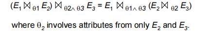
- Theta joins are associative in the following manner:
![database161]()
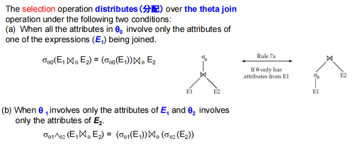
- selection distributes:
![database162]()
- projection distributes
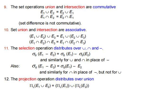
- the equivalence rules about set
![database163]()
statictics for cost estimation
statistical information for cost estimation
- nr: number of tuples in relation r
- br: number of blocks in relation r
- lr: size of tuples in relation r
- V(A,r): number of distinct values that appear in r for attribute A
selection size estimation
- $\rho_{A=v}(r)$
- $\frac{nr}{V(A,r)}$: estimate the number of tuples in r that satisfy the selection condition.
- $\rho_{A \le v}(r)$
- Let c denote the estimated number of tuples satisfying the condition.
- $c=n_r*\frac{v-min(A,r)}{max(A,r)-min(A,r)}$
size estimation of complex selections- The selectivity(中选率) of a condition $\theta_i$ is the probability that a tuple in the relation r satisfies $\theta_i$
- conjunction:$\rho_{\theta_1 \land \theta_2….}(r)$.Thus, the result is $n_r$ *
$\frac{S_1S_2S_n}$ - disjunction:$\rho_{\theta_1 \lor \theta_2….}(r)$.Thus, the result is $n_r (1-(1-\frac{S_1}{nr})(1-\frac{S_2}{nr})….)$
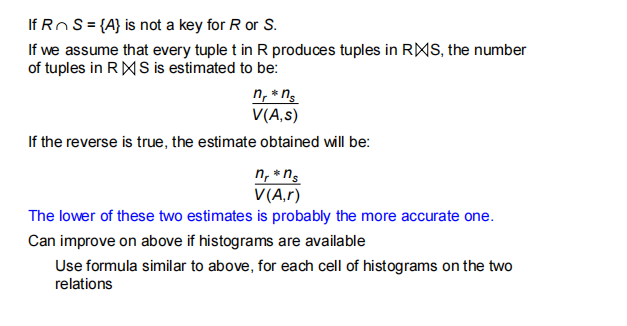
Estimation of the size of joins
choice of evaluation plans
cost-based join-order selection
想要找到最好的方式将n个表连接起来,我们有许多种选择方式。
Join Order Optimization Algorithm1
2
3
4
5
6
7
8
9
10
11
12
13
14
15procedure findbestplan(S)
if (bestplan[S].cost )
return bestplan[S]
// else bestplan[S] has not been computed earlier, compute it now
if (S contains only 1 relation)
set bestplan[S].plan and bestplan[S].cost based on the best way of accessing S using selections on S and indices (if any) on S
else for each non-empty subset S1 of S such that S1 != S
P1= findbestplan(S1)
P2= findbestplan(S - S1)
for each algorithm A for joining results of P1 and P2
… compute plan and cost of using A (see next page) ..
if cost < bestplan[S].cost
bestplan[S].cost = cost
bestplan[S].plan = plan;
return bestplan[S]cost of optimization- 在使用优化的动态规划中,时间复杂度变为$O(3^n)$
- 如果我们只考虑寻找最优的left-deep trees,那么时间复杂度变为$O(n*2^n)$
Additional Optimization Techniques
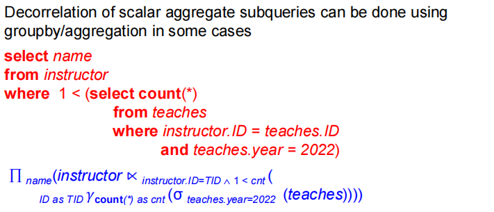
Optimizing Nested Subqueries
- 通常将嵌套查询转化为连接,降低成本
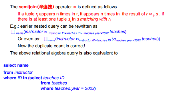
半连接优化exists的嵌套子查询- 半连接本质上和连接的差距就是只满足一边的情况,所以就适合处理嵌套子查询(只用满足嵌套子查询的条件即可)
![database165]()
- 逆半连接可以用来优化:not exists的嵌套子查询
- 半连接本质上和连接的差距就是只满足一边的情况,所以就适合处理嵌套子查询(只用满足嵌套子查询的条件即可)
处理更复杂的嵌套子查询,可能涉及分组使用聚合函数等操作![database166]()
Materialized views
- 将传统的view实际存储
- 保持物化视图与底层数据同步的任务称为物化视图维护
- Materialized views can be maintained by 、recomputation on every update. A better option is to use incremental view maintenance
Chapter 17-Transactions
Transaction Concept
- 事务是程序执行的单元,它访问并可能更新各种数据项
- 性质(ACID)
- 原子性(atomicity):事务包含的数据库操作,要么全部做,要么都不做。
- 一致性(consistency):事务执行之前和之后,数据库的完整性没有改变。
- 隔离性(isolation):事务执行过程中,其他事务不能被其他事务干扰。
- 持久性(Durability):在事务成功完成之后,它对数据库所做的更改会持续存在,即使出现系统故障。
A simple transaction model
事务对于数据的操作基于两个操作:read 和 write
example of fund transfer
- 事务:
1
2
3
4
5
6
71. read(A)
2. A := A – 50
3. write(A)
-----------------------
4. read(B)
5. B := B + 50
6. write(B)- 原子性要求:系统应确保未完全执行的交易更新不会反映在数据库中
- 持久性要求:一旦用户已被告知交易已完成(即,50美元的转账已经完成),则必须对数据库进行更新,即使发生软件或硬件故障,这些更新也必须持续。
Transaction State
- Active:初始状态
- Partially commited
- Failed
- Aborted:事务回滚后,数据库恢复到事务开始前的状态。事务被中止后有两种选择:重新启动事务和终止事务
- Commited
Concurrent Executions
- 系统允许多个事务并发执行
- advantages:提高了事务的吞吐量
- advantages:减少了事务处理的平均响应时间:短事务不必等待长事务。
Anomalies in Concurrent Executions
- Lost Update(丢失修改):几乎同时两个事务对同一个数据修改时,另外一个事务看见的数据仍然是旧的数据,所以最终丢失了修改。
- Dirty Read(脏读):当一个事务进行修改并将数据写出去后,此时另一个事务读到的是第一个事务的脏数据,但是在后面第一个事务roll back。也就是一个事务读了另一个未提交事务的数据就叫做脏读。
- Unrepeatable Read(不可重复读):当一个事务读到数据后,此时另一个事务修改了数据,那么第一个事务读到的数据可能就不再是同一个数据。
- Phantom Problem(幽灵问题):其实也是和不可重复读异曲同工,只是现在是整个表出现了更新,对于表查询结果前后出现差异。
Schedules
- 调度程序-一系列指令,用于指定并发事务的指令执行顺序
Serializability(可串行化)
- A (possibly concurrent) schedule is serializable if it is equivalent to a serial schedule.
conflict serializability
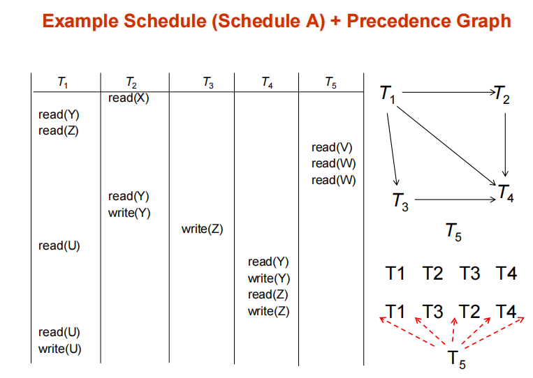
- 利用前驱图检测可串行化(如果两个事务冲突,我们从Ti到Tj绘制一条弧线,Ti访问了冲突发生较早的数据项)
- 只要前驱图不存在环,那么就是冲突可串行化的。并且等价的串行可以通过拓扑排序得到。
- example
![database171]()
View Serializability
- 设S和S‘是具有相同事务集的两个调度。如果满足下列三个条件,对于每个数据项Q,S和S’是视图等价的。
- 1.如果在调度S中,事务Ti读取了Q的初始值,则在调度S‘中,事务Ti也必须读取Q的初始值。
- 2.如果在调度S中,事务Ti执行了读取(Q),而该值是由事务Tj(如果有)产生的,那么在调度S’中,事务Ti也必须读取由事务Tj的相同写入(Q)操作产生的Q的值。
- 3.在调度S中执行最终写入(Q)操作的事务(如果有)也必须在调度S‘中执行最终写入(Q)操作。
- 如果一个调度视图等价于一个串行调度则说明它是view serializability。
Recoverable Schedules
- 可恢复的计划(可恢复调度)——如果事务Tj读取了之前由事务Ti写入的数据项,那么Ti的提交操作出现在Tj的提交操作之前
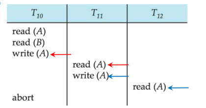
Cascading Rollbacks
- 级联回滚-单个事务失败会导致一系列事务回滚。考虑以下时间表,其中没有任何事务已提交(因此该时间表是可恢复的)
![database172]()
- 假设事务T1失败,那么事务T2和T3都将roll back。(可能导致大量工作取消)
Transaction Isolation Levels
- Serializable
- Repeatable Read:only commited records to be read,对同一记录的重复读取必须返回相同的值。但是,事务可能不是串行的–它可能找到由事务插入的某些记录,但找不到其他记录。
- Read Committed:只能读取已提交的记录,但连续读取记录可能会返回不同的(但已提交的)值
- Read Uncommitted:可以读取未提交的记录。
Chapter 18-Concurrency Control
Lock-Based Protocols
- 锁是一种机制,用于控制对数据项的同时访问。
- 数据项可以以两种模式锁定:
- 1.exclusive mode(X)。数据项既可读也可写。使用lock-X指令请求X锁。
- 2.共享(S)模式。数据项只能读取。使用lock-S指令请求S锁。
- 锁请求需提交给并发控制管理器。事务只有在请求被批准后才能继续进行。
- 如果请求的锁与其他事务已持有的锁兼容,事务可以被授予对某个项目的锁定。任意数量的事务可以持有**共享锁(S),但如果任何事务对该项目持有独占锁(X)**,则其他事务不得对该项目持有任何锁。如果无法授予锁,请求事务将等待,直到所有其他事务持有的不兼容锁都被释放。然后才会授予锁。
The Two-Phase Locking (2PL) Protocol
- Phase 1:Growoing Phase:事务获取锁,事务不能释放锁,其中Lock point为事务获取最后一个锁的时刻。
- Phase 2:Shrinking Phase:事务释放锁,事务不能获取锁
- 两阶段锁定协议保证了序列化,可以证明事务按照其锁定点的顺序进行序列化
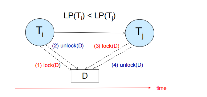
利用前驱图反证协议的正确性
- 我们现在研究两个事务,Ti,Tj.假设在前驱图上Ti有一条弧线指向Tj
- 如图所示
![database173]()
解释:因为两者发生冲突,根据Two-Phase Locking协议,当Ti进行phase2的时候,Tj才能加锁。所以两者的lock point在时间上存在先后顺序。我们可以显然得到前驱图上面没有环状结构,所以一定是conflict serializable。
继续探究2PL
- 扩展基本的两阶段锁定(基本两阶段封锁)以确保恢复自由,防止级联回滚。
- 级联回滚是指:一个事务(T1)的回滚导致其他事务(T2, T3,…)也必须回滚的现象。根本原因:事务T1释放了某些锁(如写锁)后,其他事务读取或修改了T1写过的数据,但之后T1回滚,导致这些事务基于”脏数据”继续执行,最终也必须回滚。
- strict two-phase locking(严格两阶段封锁):事务必须持有其所有exclusive锁直到提交或回滚。确保恢复并避免级联回滚。
- rigorous two-phase locking(强两阶段封锁):事务必须持有所有锁直到提交或回滚。事务可以按照提交的顺序进行序列化。
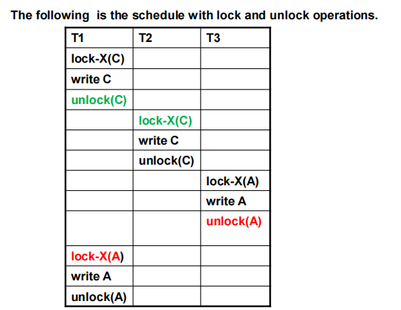
- Two-phase locking is not a necessary condition for serializability
![database181]()
如上图所示,上面例子的调度是conflict serializable,但是对于事务1并没有采用两阶段封锁协议,因为我们在释放锁后又重新获得了锁 - 两阶段封锁协议还可以进行扩展,with lock conversion
- First Phase:
can acquire a lock-S or lock-X on a data item
can convert a lock-S to a lock-X
(lock-upgrade) - Second Phase:
can release a lock-S or lock-X
can convert a lock-X to a lock-S - 从第二阶段开始,我们不能再获取锁,只能进行降级操作,所以本质上还是基础的两阶段封锁协议。
- First Phase:
implementation of locking
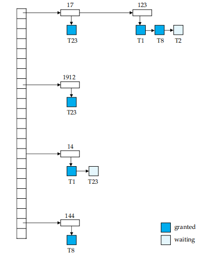
Lock Table
- Lock Table是实现Lock manager的重要数据结构,它存储了所有锁的信息。
![database182]()
- 每个记录的 id 可以放进哈希表。
- 如这里记录 123, T1、T8 获得了 S 锁,但 T2 在等待获得 X 锁。
- T1: lock-X(D) 通过 D 的 id 找到哈希表上的项,在对应项上增加。根据是否相容决定是获得锁还是等待。unlock 类似,先找到对应的数据,拿掉对应的项。同时看后续的项是否可以获得锁。
- 如果一个事务 commit, 需要放掉所有的锁,我们需要去找。因此我们还需要一个事务的表,标明每个事务所用的锁。
Deadlock Handling
Deadlock
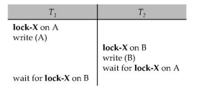
- 两个事务互相等待对方释放锁,每个事务只获取了一部分的锁,没能获取所有的锁。
- Two-phase locking does not ensure freedom from deadlocks,就如同上面的例子:当我们采用两阶段封锁协议的时候,因为我们都是执行写操作,所以必须获得X锁。但此时T1有数据A的X锁,T2有数据B的X锁,T1等待T2释放B的X锁,T2等待T1释放A的X锁。又因为两阶段封锁协议,如果我们释放锁了就不能再获得锁,所以两个事务互相等待。
Handling
- Deadlock prevention protocols ensure that the system will never enter into a deadlock state. Some prevention strategies :
- Require that each transaction locks all its data items before it begins execution (predeclaration).在执行前一次获得所有的锁
- Impose partial ordering of all data items and require that a transaction can lock data items only in the order specified by the partial order (graph-based protocol).也就是说,数据项之间存在偏序关系,事务只能按照偏序关系来锁定数据项。
- 我们也可以在等待时间上面做文章:事务只等待指定时间的锁定。之后,等待超时,事务回滚。
Deadlock Detection
- Deadlocks可以用wait-for graph描述:顶点表示所有事务,对于边:如果Ti→Tj位于E中,则存在从Ti到Tj的有向边,这意味着Ti正在等待Tj释放数据项。(边的意义主要表示的是等待关系,而前面提及的前驱图的边的关系表示的是执行顺序)
- 当Ti请求Tj当前持有的数据项时,会在等待图中插入边Ti Tj。只有当Tj不再持有Ti需要的数据项时,才会删除这条边。
- 只有当等待图中存在循环时,系统才会处于死锁状态。必须定期调用死锁检测算法来查找循环。
Deadlock Recovery
- 检测到死锁时:某些事务将不得不回滚(成为受害者)以打破死锁。选择将产生最低成本的事务作为受害者。
Graph-Based Protocols
- 协议基于的思想:在数据项集合D = {d1,d2 ,…,dh }上施加部分排序→。如果di→dj,则访问di和dj的任何事务都必须先访问di,再访问dj。这意味着集合D现在可以被视为一个有向无环图,称为数据库图。
Tree Protocol
- The tree-protocol is a simple kind of graph protocol.
- Only exclusive locks are allowed.只有X锁允许。
- The first lock by Ti may be on any data item. Subsequently, a data Q can be locked by Ti only if the parent of Q is currently locked by Ti.第一个锁可以放任意地方,后面的锁只能在父节点锁住时才能往下锁。
- Data items may be unlocked at any time.
- A data item that has been locked and unlocked by Ti cannot subsequently be relocked by Ti.放了之后不能再加锁了。
- The tree protocol ensures conflict serializability as well as freedom from
deadlock.(很容易想到,因为树协议避免死锁的本质是:它强制事务按照树的结构“向下”加锁,并禁止回头,从而破坏了死锁所需的循环等待条件。) advatange:- 在树锁定协议中,解锁可能比在两阶段锁定协议中更早发生。缩短等待时间更短,提高并发性协议
- 无死锁,不需要回滚
disadvantage:- 协议不保证可恢复性(不能从未提交的事务读取数据)或级联自由:需要引入提交依赖关系以确保可恢复性事务
- 可能需要锁定比实际需要更多的数据项(对于某个操作,你必须要锁住这个数据项的依赖关系上的“祖先”):增加锁定开销和额外等待时间,并发性可能降低
Multiple Granularity
- 多粒度锁协议主要解决以下两个问题:
- 在层级结构中支持不同粒度的锁操作
- 在不违反一致性的前提下,提高并发性
- 避免死锁,并保证可串行化
- 可以锁在记录上(如 update table set …;),也可以锁在整个表上(如 select * from table;)。
- Granularity of locking (level in tree where locking is done):
- fine granularity(细粒度) (lower in tree): high concurrency, high locking overhead
- coarse granularity(粗粒度) (higher in tree): low locking overhead, low concurrency
level
- 自上而下的level:
- database
- area
- File
- record
Intention lock Modes
intention-shared (IS): indicates explicit locking at a lower level of the tree but only with shared locks.
intention-exclusive (IX): indicates explicit locking at a lower level with exclusive or shared locks
shared and intention-exclusive (SIX): the subtree rooted by that node is locked explicitly in shared mode and explicit locking is being done at a lower level with exclusive-mode locks.
如果一个事务要给一个记录加 S 锁,那也要在表上加 IS 锁。(意向共享锁)
如果一个事务要给一个记录加 X 锁,那也要在表上加 IX 锁。(意向排他锁)
SIX 锁是 S 和 IX 锁的结合。要读整个表,但可能对其中某些记录进行修改。(共享意向排他)
这样当我们想向一个表上 S 锁时,发现表上有 IX 锁,这样我们很快就发现了冲突,需要等待。IS 和 IX 是不冲突的。在表上是不冲突的,可能在记录上冲突(即对一个记录又读又写,冲突发生在记录层面而非表)。
表格
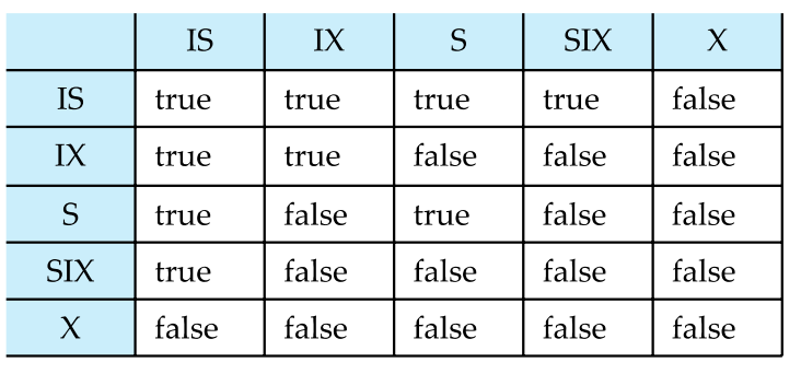
锁类型 含义 作用 S(Shared)共享读 允许多个读 X(Exclusive)排他写 读写都独占 IS(Intention Shared)意向共享 表示将对子节点加 S/IS 锁 IX(Intention Exclusive)意向排他 表示将对子节点加 X/SIX/IX/IS/S 锁 SIX(Shared + Intention Exclusive)当前节点 S,子节点可能加排他锁 少见但用于提升并发,表示将对子节点加 X/SIX/IX/S/IS 锁 相容矩阵
![database184]()
多粒度枷锁协议
- 遵守锁兼容性矩阵:所有加锁行为必须查表,不能违反冲突关系。
- 必须先锁根节点,可以是任意锁模式:所有加锁路径必须从树的顶端(根)开始。构成自顶向下的锁定路径。
- 要在某节点 Q 加 S 或 IS 锁,Ti 必须持有 Q 的父节点的 IS 或 IX 锁:表示你只想读或打算向下加读锁 ⇒ 父节点也必须表示“我在下面要读”,避免冲突
- 要在 Q 加 X、IX 或 SIX 锁,父节点必须被 Ti 持有 IX 或 SIX 锁:意思是你要对 Q 做“排他性”操作 ⇒ 父节点也要“声明我会排他地访问后代”
- 遵守两阶段锁协议(2PL):加锁之后不能再加锁,只能释放锁:加锁必须在前半阶段完成,确保事务串行化
- Ti 只能释放 Q 的锁当且仅当它不再锁定 Q 的任何子节点:避免释放父节点后,子节点的访问不再合法(保持一致性)